Hopfield Network

Introduction to networks

The general description of a dynamical system can be used to interpret complex systems composed of multiple subsystems. In this way, we can model and understand better complex networks. The first building block to describe a network is the concept of the feedback loop.

A simple system with scalar input and outputs, with a feedback loop, can be represented in the following way:

where $\bar{u}_1$ is the input function of the closed-loop system, $y_1$ is the output of the closed-loop system, $u_1$ is the input to the open-loop subsystem, $S_1$ is the open-loop subsystem, $S^*_1$ is the feedback loop subsystem and $y^*_1$ is the output of the feedback loop. The above system is a Single In Single Output system. More complex type of system present multiple inputs and multiple outputs. The following scheme is a system of that type and represents the prototype of the Hopfield Network, namely is a network where each building book outputs influences the inputs of the others.  

The Hopfield Network

The Hopfield Network is a complex system, made of multiple interconnected non-linear subsystems, that serves as a model for associative memory of our brain. We will call these subsystems artificial neurons because they mimic the behaviour of neurons in our brains. 

To see how to build a Hopfield Network we can start from the previous diagram and simplify it setting $\bar{u}_1=\bar{u}_2=0$  and defining the feedbacks subsystems as $S^*_i:\; y^*_i=w_{ij}\cdot y_i$. Then we increase the number of "nodes" (i.e. subsystems/neurons) so that every neuron output influences the input of other neurons:

So finally the generic $u_i$ input reads (adding a scalar bias to each neuron)

$$ u_i =   \sum_{j=0}^m w_{ij} y_j+b_i .$$ In the Hopfield Network the matrix $w_{ij} = w_{ji}$ is symmetric and neurons don't have a self-feedback ($w_{ii}=0$).

The Artificial Neuron

Now, let's see how an artificial neuron behaves. The biological neurons work as on/off switchers of signals. When a neuron receives sufficient stimulation from his receptors it fires an output signal. This behaviour is described by a non-linear activation function usually represented by a sigmoid-shaped function. In artificial neurons, usually, its behaviour is idealised using the sign function.

We can write the i-th neuron output as

$$ y^{[t+1]}_i =  \Theta \left( \sum_{j=0}^m w_{ij} y^{[t]}_j +b_i\right).$$

where $\Theta$ is a non linear activation function and $b_i$ is a scalar bias characteristic of each neuron. Regarding the state of a neuron we have a bit of freedom: either we set it to be its state of excitement (i.e. $s^{[t+1]}_i= u^{[t]}_i=\sum_{j=0}^m w_{ij} y^{[t]}_j +b_i$) or more simply we set it to be equal to the output  (i.e. $s^{[t+1]}_i= y^{[t+1]}_i $)  . 

Hopfield Network "Energy" and convergence

After defining the state of the Hopfield's Network to be the collection of states of every neuron (outputs) $\mathbf{s}=\left\{ y_{1},\ldots,y_{N}\right\}=\left\{ s_{1},\ldots,s_{N}\right\}$, we want to show that at some point the system state will stop to evolve and it will reach a steady state. 

To do so we first note that that

$$ if\quad\Theta=\mathrm{sign}()\quad\Rightarrow\quad y_{i}^{[t]}=\begin{cases} 1\\ -1 \end{cases},\quad\left(y_{i}^{[t+1]}-y_{i}^{[t]}\right)=\begin{cases}0 \\ 2y_{i}^{[t]} \end{cases} $$

$$\Rightarrow\quad y_{i}^{[t+1]}u_{i}^{[t]}-y_{i}^{[t]}u_{i}^{[t]}=\left(y_{i}^{[t+1]}-y_{i}^{[t]}\right)u_{i}^{[t]}=\begin{cases} 0\\ 2y_{i}^{[t]}u_{i}^{[t]} \end{cases}\geq 0 $$

this means that the change of state of the neuron $i$ neuron cannot decrease the value of $u_i y_i$. Summing up over all neurons (but avoiding double counting of some terms):

$$ D\left(y_{1}^{[t]},\ldots,y_{i}^{[t]},\ldots,y_{N}^{[t]}\right)=\sum_{i}y_{i}^{[t]}\left(\sum_{j<i}w_{ji}y_{j}^{[t]}+b_{i}\right) $$

if one of the N neurons changes states we have again that

$$ \Delta D^{y_{i}^{[t]}\to y_{i}^{[t+1]}}=D\left(y_{1}^{[t]},\ldots,y_{i}^{[t+1]},\ldots,y_{N}^{[t]}\right)-D\left(y_{1}^{[t]},\ldots,y_{i}^{[t]},\ldots,y_{N}^{[t]}\right)\geq 0. $$

 Therefore we conclude that $\Delta D^{t\to t+1}\geq 0$. We can give a physical interpretation defining the system energy $E=-D\leq 0$ and saying that the Hopfield Network evolves minimizing its energy $E$.

Finally, proving that the energy $E$ is bounded 

$$ E_{{\rm min}}=-\sum_{i}\left(\sum_{j<i}\left|w_{ji}\right|+\left|b_{i}\right|\right) $$  we can say that the system will converge after a finite number of steps.

Note that the weights matrix $w_{ij}$ gives the "shape" to the energy landscape of the network, while the state $\mathbf{s}$ serves as "coordinate" in the energy landscape.

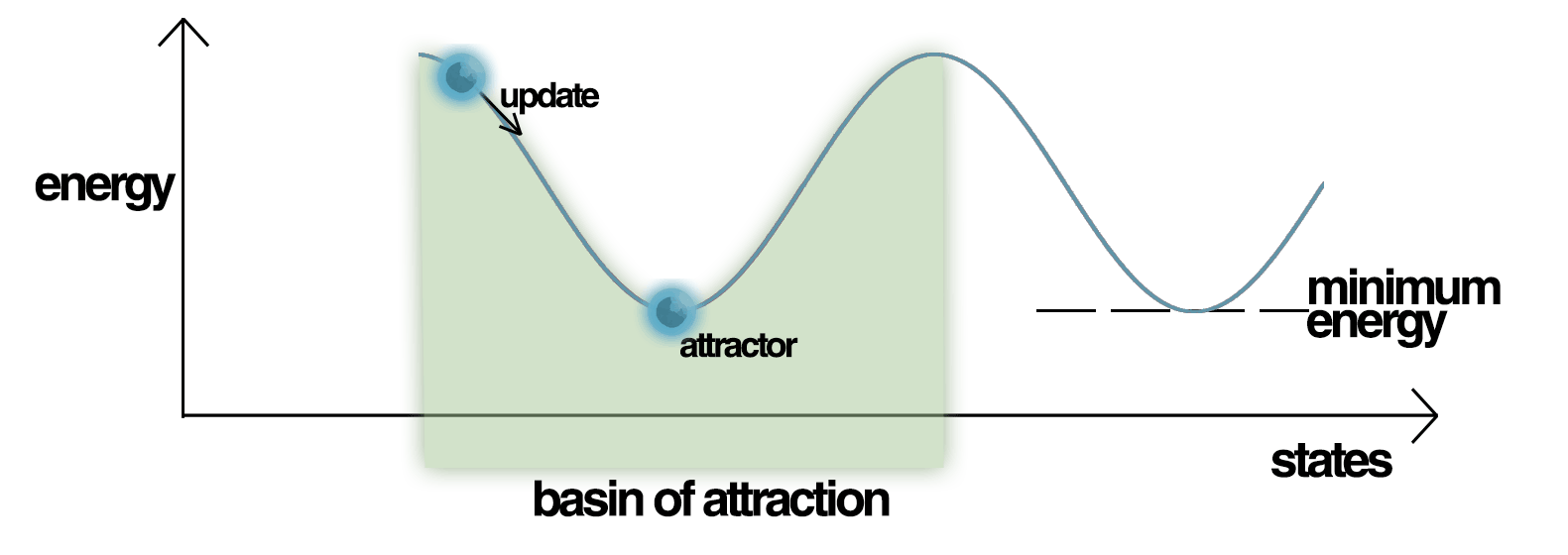
Wikipedia figure -  Energy Landscape of a Hopfield Network, highlighting the current state of the network (up the hill), an attractor state to which it will eventually converge, a minimum energy level and a basin of attraction shaded in green. Note how the update of the Hopfield Network is always going down in Energy.

Shaping matrix W to store information: Hebbian theory

As previously mentioned, the landscape of the energy function of the network is correlated to the values of the weighting matrix

$$ E^{[t]}=-\sum_{i}y_{i}^{[t]}\left(\sum_{j<i}w_{ji}y_{j}^{[t]}+b_{i}\right)\ . $$

We have seen in particular that its minimum is completely defined by the weights and the biases

$$ E_{{\rm min}}=-\sum_{i}\left(\sum_{j<i}\left|w_{ji}\right|+\left|b_{i}\right|\right) $$

Therefore, carefully choosing the biases and the weights we can shape of $E$ assigning a minimum energy to well-defined states of the network (attractor points). In this way, our network can recover its original state if it is perturbed from the equilibrium point.

The Hebbian theory gives us a way to shape the weighting matrix. In practice, this theory leads to Hebb's rule to create an attractor in the energy landscape:

$$w_{ij} = \frac{1}{N}  s^*_i s^*_j,$$

where $\mathbf{s}^* = \left\{ s^*_1,\ldots,s^*_N\right\}$ is the attractor state. This simple rule can then be extended to shape an Energy landscape with multiple attractors

$$w_{ij} = \frac{1}{N} \sum_{K=1}^p s_i^K s_j^K$$ where $ \mathbf{s}^K=\{ s_{1}^K,\ldots,s_{N}^{K}\} $ is the $K-th$ attractor state. Mind that 

$$  s_{i}^{K}s_{j}^{K}=\left[\begin{array}{ccc} s_{1}^{K}s_{1}^{K} & \cdots & s_{1}^{K}s_{N}^{K}\\ \vdots & \ddots & \vdots\\ s_{N}^{K}s_{1}^{K} & \cdots & s_{N}^{K}s_{N}^{K} \end{array}\right] $$